L3

last lecture :Linear model $\hat y=x*w$

梯度下降

**optimization Problem 优化问题

Gradient Descent Algorithm 梯度下降

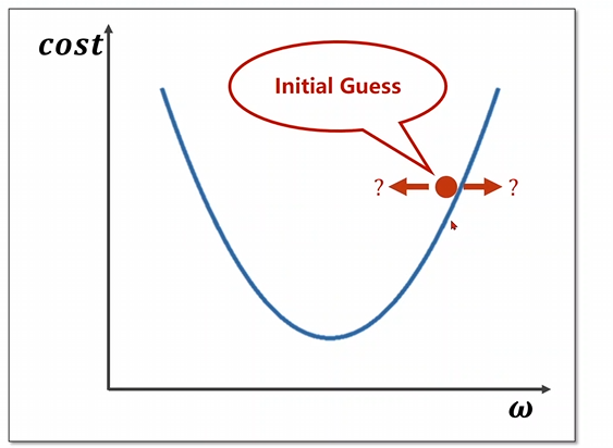
Grandient $\frac{\partial cost}{\partial w}$ Update $w=w-\alpha\frac{\partial cost}{\partial w}$ 每一次迭代都朝向下降最快的方向走一步 贪心算法 找到局部最优解 但无法找到全局最优解

• 鞍点 **梯度为0的点 并没有局部最优解 如果我们到达了这一点 使得我们的梯度无法再次下降 Repeat Gradient Descent $\frac{\partial cost}{\partial w}=\frac{\partial}{\partial w}*\frac{1}{N}\sum_{n=1}^{N}(x_n*w-y_n)^2\\=\frac{1}{N}\sum_{n=1}^{N}*\frac{\partial}{\partial w}*(x_n*w-y_n)^2\\=frac{1}{N}\sum_{n=1}^{N}2*(x_n*w-y_n)\frac{\partial (x_n*w-y_n)}{w}\\=\frac{1}{N}\sum_{n=1}{N}2*x_n*(x_n*w-y_n)$ Update $w=w-\alpha*\frac{1}{N}\sum_{n=1}{N}2*x_n(x_n*w-y_n)$

x_data={1.0,2.0,3.0}
y_data={2.0,4.0,6.0}

#inital guess
w=1.0

def forward(x)
	return x*w
def cost(xs,ys)
	cost=0
		for x,y in zip(xs,xs):
			y_pred=forward(x)
			cost+=(y_pred-y)**2
		return cost/len(xs)
def gradient(xs,ys):
	grad=0
	for x,y in zip(xs,ys):
		grad+=2*x*(x*w-y)
	return grad/len(xs)
print('Predict (before training)',4,forward(4))

for epoch in range (100):
	cost_val=cost(x_data,y_data)
	grad_val=gradient(x_data,y_data)
	w-=0.01*grad_val
	print('Epoch:',epoch,'w=:'w,'loss=',cost_val)
print('Predict after training',4,forward(4))

对costfunction 进行绘图的时候 有时候噪声很大 我们可以对costfunction进行指数加权均值叠加 使之变得平滑 Gradient Descent $w=w-\alpha*\frac{\partial cost}{\partial w}$ Stochastic Gradient Descent 随机梯度下降 $w=w-\alpha*\frac{\partial loss}{\partial w}$ 用单个样本的损失对w进行梯度下降 Derivative of Cost Function $\frac{\partial cost}{\partial w}=\frac{1}{N}\sum_{n=1}^{N}2*x_n*(x_n*w-y_n)^2$ Derivative of Loss Function $\frac{\partial loss}{\partial w}=2*x_n*(x_n*w-y_n)^2$

#Stochastic Gradient Descent 
x_data={1.0,2.0,3.0}
y_data={2.0,4.0,6.0}

#inital guess
w=1.0

def forward(x)
	return x*w
#这次我们只选择单个样本
def cost(xs,ys)
		y_pred=forward(x)
		return (y_pred-y)**2
def gradient(xs,ys):
	return 2*x*(x*w-y)
print('Predict (before training)',4,forward(4))

for epoch in range (100):
	for x,y in zip(x_data,y_data):
	grad=gradient(x,y)
	w-=0.01*grad
	print('\tgrad',x,y,grad)
print('Predict after training',4,forward(4))

**在原本的梯度下降中训练过程中$f(x_i)\,f(x_{i+1})$并没有什么依赖关系 意味这这些运算都是可以并行的 但是随机梯度下降则不行因为$w-=\alpha*\frac{\partial g(x_i)}{\partial w}$和$w-=\alpha*\frac{\partial g(x_i+1)}{\partial w}$二者之间存在依赖关系 则不能并行运算

Stochastic Gradient Descent	Gradient Descent
性能低	高
时间复杂度低	高
在性能和时间复杂度中折中 我们对选择一个Batch 每次选择一个batch中几个并行 从而对时间复杂度和性能取折中 最开始的Batch指的是全部 更正式的名字是Mini-Batch 小批量的