
Last Lecture
Linear model **input x 权重x Stochastic Gradient Descent Derivative Gradient Descent
复杂的神经网络
- **Gradient 对于hiddenlayer较多的神经网络 需要的输入输出权重极多
Computational Graph
手绘图源文件:Drawing 2026-04-17 23.19.30.excalidraw
Book->Martix cookbook
无论多少层都可以化简为一个简单的线性模型 但我们希望模型可以愈加复杂 提高模型的复杂度 但增加权重函数没有意义 因而我们可以增加非线性函数打破这种化简的规律 例如sigmond函数
Composition of functions and Chain Rules
**Chain rules 手绘图源文件:Drawing 2026-04-18 16.29.26.excalidraw
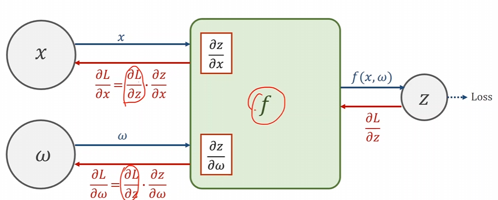
有同学可能说并没有什么需求 但是要是这里的x是一个中间变量
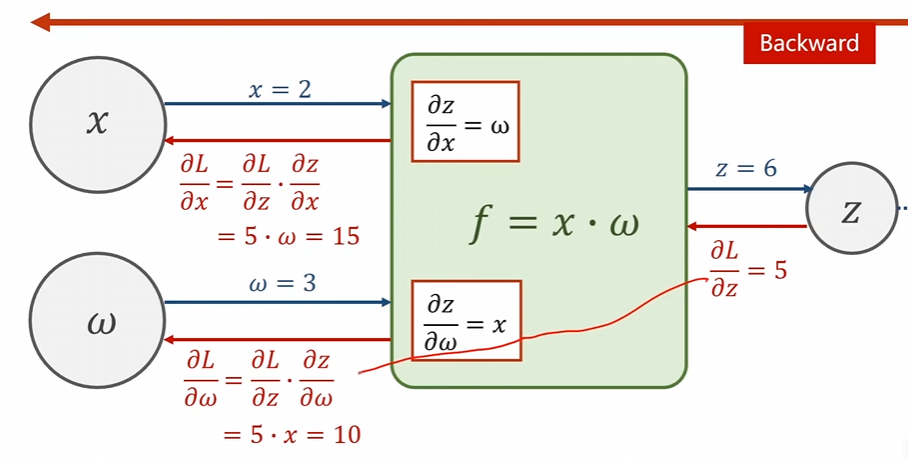
Computational Graph of Linear Model
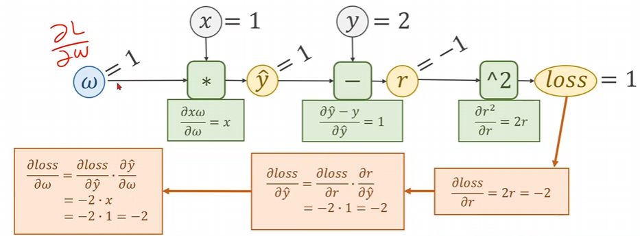
**Practice:
- x= 2,y=4 重新计算反向传播
- Affine Model :
Tensor in Pytorch
**In pytorch,Tensor is the important compenant in constructing dynamic computational graph It contains data and grad,which storage the value of node and gradient w.r.t loss respectively.
import torch
x_data =[1.0,2.0,3.0]
y_data =[2.0,4.0,6.0]
w=torch.Tensor([1.0])
w.requires_grad=True#需要计算梯度
if autograd mechanics are required,the element variable requires_grad of Tensor has to be set to True 默认tensor计算过程中requires_grad是False,不会去保留关于w的梯度
def foeward(x):
	return x*w
def loss(x,y):
	y_pred=forward(x)
	return (y_pred-y)**2
这里的w是一个Tensor x和w要进行数乘 因而x需要进行自动类型转换
print("predict (before training)",4,forward(4).item)

for epoch in range(100):
	for x,y in zip(x_data,y_data):
		#compute the forward
		l=loss(x,y)
		#backward computre grad for Tensor whose requires_grad set True
		l.backward()
		print('\tgrad',x,y,w.grad.item())
		w.data=w.data-0.01*w.grad.data
		#The grad computed by .bacjward() will be accumulated So after update,remember set the grad to Zero
		w.grad.data.zero_()
	print("progress:",epoch,1.item())
print("predict (after training)",4,forwarda(4).item())
我们每调用一次loss函数 就将这个计算图动态构建出来 因而每次看见这个代码 就能够构建一次这个计算图 但是每一次backward时候就会将计算图释放掉而去准备下一次的图 因而下一次调用loss函数时会创建一个新的计算图 这是一个非常灵活的方式 也是pytorch的核心竞争力
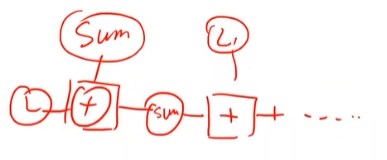
sum=0
sum+=l

sum+=l.item
**由于没有backward操作释放计算图 因而所有计算图一直保留 在内存中从而使使得内存容量爆炸 因为这里的l是一个Tensor Tensor在进行加法计算时 会构建计算图 **
Practice:
**Input:Quadartic Model Loss Function:
x_data=[1.0,2.0,3.0]
y_data=[2.0,4.0,6.0]
尝试利用pytorch实现