处理多维特征的输入

Diabetes Dataset

每一行是Sample 每一行是Feature **原来:Logistic Regression Model $\hat y^{(i)}=\sigma(x^{i}*w+b)$ **现在:Logistic Regression Model $\hat y^{(i)}=\sigma(\sum_{n=1}^{8}x_{n}^{(i)}*w_n+b)$ **习惯上我们叫这部分$z^{(i)}$

$$\sum_{n=1}^{8}\newline \begin{bmatrix} x_{1}{(i)}\,...\,x_{8}^{(i)} \end{bmatrix}*\newline \begin{bmatrix} w_{1}\\ ...\\ w_{8} \end{bmatrix}$$

**实际的Logistic Regression Model

$$\begin{align} \hat y^{(i)}=\sigma(\begin{bmatrix} x_{1}{(i)}\,...\,x_{8}^{(i)} \end{bmatrix}* \begin{bmatrix} w_{1}\\ ...\\ w_{8} \end{bmatrix}+b)=\sigma(z^{(i)}) \end{align}$$

Mini-Batch(N samples)

**Sigmond function is in an element-wise fashion

$$\begin{bmatrix} \hat y^{(1)}\\ ...\\ \hat y^{(N)} \end{bmatrix}= \begin{bmatrix} \sigma(z^{(1)})\\ ...\\ \sigma(z^{(N)}) \end{bmatrix}= \sigma(\begin{bmatrix} z^{(1)}\\ ...\\ z^{(N)} \end{bmatrix})$$ $$\begin{align} z^{(1)}= \sum_{n=1}^{8} \begin{bmatrix} x_{1}^{(1)}\,...\,x_{8}^{(1)} \end{bmatrix}* \begin{bmatrix} w_{1}\\ ...\\ w_{8} \end{bmatrix} \newline ...\newline z^{(n)}= \sum_{n=1}^{8} \begin{bmatrix} x_{1}^{(N)}\,...\,x_{8}^{(N)} \end{bmatrix}* \begin{bmatrix} w_{1}\\ ...\\ w_{8} \end{bmatrix} \end{align}$$

**So we get:

$$\begin{bmatrix} z^{(1)}\\ ...\\ z^{(N)} \end{bmatrix}= \begin{bmatrix} x_{1}^{(1)}\,...\,x_{8}^{(1)}\\ ...\,...\,...\\ x_{1}^{(N)}\,...\,x_{8}^{(N)} \end{bmatrix}+ \begin{bmatrix} b\\ ...\\ b \end{bmatrix}$$

class Model(torch.nn.Module):
    def __init__(self):
    #我们只是把Linaer改成8*1
    super.linear=torch.nn.Linear(8,1)
    self.sigmond=torch.nn.Sigmoid()
    
    def forward(self,x):
    x=self.sigmond(self.linear((x))
    return x
model = Model()

self.linear=torch.nn.Linear(8,2)

Linear Layer

降维

**8代表8维输入例如$x_{1}...x_{8}$ 2代表2维输出 Linear至少可以做到空间输入的变换 从而实现到降维的目的 我们最终的目标可能是8Dim->1Dim 所以我们可以引入激活函数为线性变换增加非线性的因子 使得我们能够拟合非线性的变换

Neural Network

**超参数的搜索方法 一般来说：hidden layer越多 越复杂 学习能力越强 但是学习能力并不是说越强越好 还需要有一定的泛化能力

ablicity:

• 扣书本
• 读文档，基本架构理念 **(泛化能力比较好)

Example:Artifical Netural Network

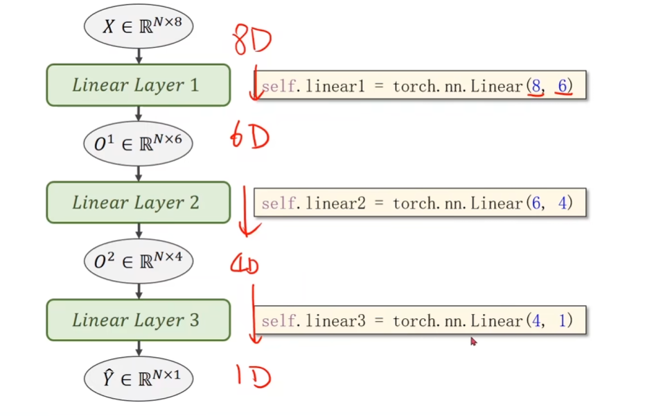
Examples:Diabetes Prediction:

• Prepare dataset

import numpy as np
xy=np.loadtxt('dibates.csv.gz',delimiter=',',dtype=np.float32)
x_data=torch.from_numpy(xy[:,:-1])
y_data=torch.form_numpy(xy[:,[-1]])

• Design model using Class

import torch

class Model(torch.nn.Module):
	def __init__(self):
		super(Model,self).__init__()
		self.linear1=torch.nn.Linear(8,6)
		self.linear2=torch.nn.Linear(6,4)
		self.linear3=torch.nn.Linear(4,1)
		self.sigmoid=torch.nn.Sigmoid()
	def forward(self,x):
		x=self.sigmoid(self.linear1(x))
		x=self.sigmoid(self.linear2(x))
		x=self.sigmoig(self.linear3(x))
		return x
model=Model()

• Construst loss and opyimizer **Mini-Batch loss Function for Binart Classification: $loss=-\frac{1}{N}\sum_{n=1}{N}y_{n}log\hat y_{n}+(1-y_{n})log(1-\hat y_{n})$ Update: $w=w-\alpha\frac{\partial cost}{\partial w}$

criterion=torch.nn.BCELoss(size_average=True)
optimizer=torch.optim.SGD(model.parameters(),lr=0.1)

• Training cycle **(前馈 反馈 更新)

for epoch in range(100):
	#Forward:
	y_pred=model(x_data)#Notoce:This program has not use Mini-Batch for training.We shall talk about Dataloader later
	loss=criterion(y_pred,y_data)
	print(epoch,loss.item())
	#Backwad
	optimizer.zero_grad()
	loss.backward()
	#Update
	optimizer.step()

Exercise:Try different activate function

#实际上我们选择不同的激活函数 每次只需要更改这一行
self.sigmoid=torch.nn.Sigmoid()
self.activate=torch.nn.ReLU()